Shear band localization

Shear band localization miniapp to test the visco-elasto-plastic rheology implementation in JustRelax.jl

Initialize packages

Load JustRelax.jl necessary modules and define backend.

using JustRelax, JustRelax.JustRelax2D, JustRelax.DataIO
using Pkg; Pkg.activate("miniapps")
const backend_JR = CPUBackend

using JustPIC
import JustPIC.GridGeometryUtils as GGU
const backend_JP = JustPIC.CPU

We will also use ParallelStencil.jl to write some device-agnostic helper functions:

using ParallelStencil
@init_parallel_stencil(Threads, Float64, 2) #or (CUDA, Float64, 2) or (AMDGPU, Float64, 2)

and will use GeoParams.jl to define and compute physical properties of the materials:

using GeoParams

Script

Model domain

nx = ny      = 64                       # number of cells per dimension
igg          = IGG(
    init_global_grid(nx, ny, 1; init_MPI= true)...
)                                       # initialize MPI grid
ly           = 1.0                      # domain length in y
lx           = ly                       # domain length in x
ni           = nx, ny                   # number of cells
li           = lx, ly                   # domain length in x- and y-
di           = @. li / ni               # grid step in x- and -y
origin       = 0.0, 0.0                 # origin coordinates
grid         = Geometry(ni, li; origin = origin)
(; xci, xvi) = grid                     # nodes at the center and vertices of the cells

Physical properties using GeoParams

τ_y     = 1.6           # yield stress. If do_DP=true, τ_y stand for the cohesion: c*cos(ϕ)
ϕ       = 30            # friction angle
C       = τ_y           # Cohesion
η0      = 1.0           # viscosity
G0      = 1.0           # elastic shear modulus
Gi      = G0 / 2        # elastic shear modulus perturbation
εbg     = 1.0           # background strain-rate
η_reg   = 8e-3          # regularisation "viscosity"
dt      = η0 / G0 / 4.0 # assumes Maxwell time of 4
el_bg   = ConstantElasticity(; G = G0, Kb = 4.0)
el_inc  = ConstantElasticity(; G = Gi, Kb = 4.0)
visc    = LinearViscous(; η = η0)
pl      = DruckerPrager_regularised(;  # non-regularized plasticity
    C    = C / cosd(ϕ),
    ϕ    = ϕ,
    η_vp = η_reg,
    Ψ    = 0
)

Rheology

rheology = (
    # Low density phase
    SetMaterialParams(;
        Phase             = 1,
        Density           = ConstantDensity(; ρ = 0.0),
        Gravity           = ConstantGravity(; g = 0.0),
        CompositeRheology = CompositeRheology((visc, el_bg, pl)),
        Elasticity        = el_bg,

    ),
    # High density phase
    SetMaterialParams(;
        Phase             = 2,
        Density           = ConstantDensity(; ρ = 0.0),
        Gravity           = ConstantGravity(; g = 0.0),
        CompositeRheology = CompositeRheology((visc, el_inc, pl)),
        Elasticity        = el_inc,
    ),
)

Phase anomaly

Helper function to initialize material phases with ParallelStencil.jl

function init_phases!(phase_ratios, xci, xvi, circle)
    ni = size(phase_ratios.center)

    @parallel_indices (i, j) function init_phases!(phases, xc, yc, circle)
        x, y = xc[i], yc[j]
        p = GGU.Point(x, y)
        if GGU.inside(p, circle)
            @index phases[1, i, j] = 0.0
            @index phases[2, i, j] = 1.0

        else
            @index phases[1, i, j] = 1.0
            @index phases[2, i, j] = 0.0

        end
        return nothing
    end

    @parallel (@idx ni) init_phases!(phase_ratios.center, xci..., circle)
    @parallel (@idx ni .+ 1) init_phases!(phase_ratios.vertex, xvi..., circle)
    return nothing
end

and finally we need the phase ratios at the cell centers:

phase_ratios  = PhaseRatios(backend_JP, length(rheology), ni)
circle_radius = 0.1
circle_origin = 0.5, 0.5
circle        = GGU.Circle(circle_origin, circle_radius)
init_phases!(phase_ratios, xci, xvi, circle)

Stokes arrays

Stokes arrays object

stokes = StokesArrays(backend_JR, ni)

Pseuo-transient coefficients

pt_stokes = PTStokesCoeffs(li, di; ϵ_abs = 1.0e-6, ϵ_rel = 1.0e-6, CFL = 0.95 / √2)

Initialize viscosity fields

We initialize the buoyancy forces and viscosity

ρg               = @zeros(ni...), @zeros(ni...)
args             = (; T = @zeros(ni .+ 2...), P = stokes.P, dt = dt)
viscosity_cutoff = (-Inf, Inf)
compute_viscosity!(stokes, phase_ratios, args, rheology, viscosity_cutoff)

where (-Inf, Inf) is the viscosity cutoff.

Boundary conditions

flow_bcs     = VelocityBoundaryConditions(;
    free_slip = (left = true, right = true, top = true, bot = true),
    no_slip   = (left = false, right = false, top = false, bot=false),
)
stokes.V.Vx .= PTArray(backend_JR)([ x * εbg for x in xvi[1], _ in 1:(ny + 2)])
stokes.V.Vy .= PTArray(backend_JR)([-y * εbg for _ in 1:(nx + 2), y in xvi[2]])
flow_bcs!(stokes, flow_bcs) # apply boundary conditions
update_halo!(@velocity(stokes)...) # if running on MPI

Just before solving the problem...

In this benchmark we want to keep track of τII, the total time ttot, and the analytical elastic solution sol

solution(ε, t, G, η) = 2 * ε * η * (1 - exp(-G * t / η))

and store their time history in the vectors:

τII        = [0e0]
sol        = [0e0]
ttot       = [0e0]

Solving Stokes

1. Solve stokes

t  = 0.0
nt = 15 # number of time steps
for it in 1:nt
    # solve Stokes equations
    solve!(
        stokes,
        pt_stokes,
        grid,
        flow_bcs,
        ρg,
        phase_ratios,
        rheology,
        args,
        dt,
        igg;
        kwargs = (
            verbose          = false,
            iterMax          = 50.0e3,
            nout             = 1.0e3,
            λ_relaxation     = 0.2, # relaxation parameter for plastic multiplier λ
            viscosity_cutoff = (-Inf, Inf),
        )
    )
    # advance time step
    t += dt
    # calculate the second invariants and push to history vectors
    tensor_invariant!(stokes.ε)
    tensor_invariant!(stokes.ε_pl)
    push!(τII, maximum(stokes.τ.xx))
    push!(sol, solution(εbg, t, G0, η0))
    push!(ttot, t)
end

Visualization

We will use Makie.jl to visualize the results

using CairoMakie

Fields

# visualisation of high density inclusion
radius = 0.1
th     = 0:pi/50:3*pi;
xunit  = @. radius * cos(th) + 0.5;
yunit  = @. radius * sin(th) + 0.5;

fig   = Figure(size = (1600, 1600), title = "t = $t")
ax1   = Axis(fig[1,1], aspect = 1, title = L"\tau_{II}", titlesize=35)
ax2   = Axis(fig[2,1], aspect = 1, title = L"E_{II}^{\text{plastic}}", titlesize=35)
ax3   = Axis(fig[1,2], aspect = 1, title = L"\log_{10}(\varepsilon_{II})", titlesize=35)
ax4   = Axis(fig[2,2], aspect = 1)
heatmap!(ax1, xci..., Array(stokes.τ.II) , colormap=:batlow)
heatmap!(ax2, xci..., Array(log10.(stokes.EII_pl)) , colormap=:batlow)
heatmap!(ax3, xci..., Array(log10.(stokes.ε.II)) , colormap=:batlow)
for ax in (ax1, ax2, ax3)
    lines!(ax, xunit, yunit, color = :white, linewidth = 3)
end
lines!(ax4, ttot, τII, color = :black)
lines!(ax4, ttot, sol, color = :red)
hidexdecorations!(ax1)
hidexdecorations!(ax3)
fig

Final model

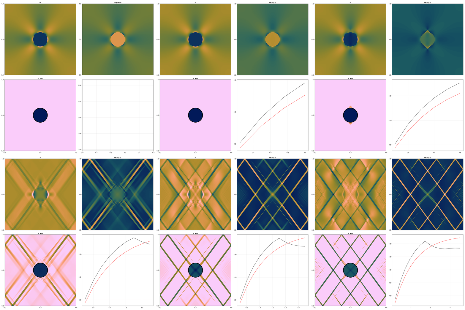
Shear Bands evolution in a 2D visco-elasto-plastic rheology model with a resolution of $2058\times 2058$ cells.