
Periodic 2D thermal diffusion
The smallest complete JustRelax.jl model: heat diffusing through a 2D slab with periodic left/right boundaries, fixed top/bottom temperatures, and a circular hot perturbation partway down. It runs on a small grid, with no particles and no separate rheology file — the natural first thing to run. For larger, physically richer setups see the Blankenbach benchmark and the other worked examples.
Set isCUDA = true to run the same model on an NVIDIA GPU.
const isCUDA = false

@static if isCUDA
    using CUDA
end

using JustRelax, JustRelax.JustRelax2D
using CairoMakie
JustRelax dispatches on a backend trait rather than the array type directly, so the same solver code runs unmodified on CPU, CUDA, or AMDGPU (see Selecting the backend).
const backend = @static if isCUDA
    JustRelax.CUDABackend # Options: CPUBackend, CUDABackend, AMDGPUBackend
else
    JustRelax.CPUBackend # Options: CPUBackend, CUDABackend, AMDGPUBackend
endCPUBackendParallelStencil generates the compute kernels for the same device.
using ParallelStencil, ParallelStencil.FiniteDifferences2D

@static if isCUDA
    @init_parallel_stencil(CUDA, Float64, 2)
else
    @init_parallel_stencil(Threads, Float64, 2)
end

using GeoParams
Initial and boundary conditions
init_T! sets a linear temperature gradient between the fixed top and bottom boundary values (300 K and 3500 K), and circular_perturbation! adds a localized hot anomaly on top of it.
@parallel_indices (i, j) function init_T!(T, z)
    if z[j] == maximum(z)
        T[i + 1, j + 1] = 300.0
    elseif z[j] == minimum(z)
        T[i + 1, j + 1] = 3500.0
    else
        T[i + 1, j + 1] = z[j] * (1900.0 - 1600.0) / minimum(z) + 1600.0
    end
    return nothing
end

function circular_perturbation!(T, δT, xc, yc, r, xci)
    @parallel_indices (i, j) function _circular_perturbation!(T, x, y)
        if (x[i] - xc)^2 + (y[j] - yc)^2 ≤ r^2
            T[i + 1, j + 1] += δT
        end
        return nothing
    end
    ni = size(T) .- 2
    return @parallel (@idx ni) _circular_perturbation!(T, xci...)
end
circular_perturbation! (generic function with 1 method)Model setup and time loop
Geometry builds the staggered grid, SetMaterialParams (from GeoParams.jl) defines the constant density, heat capacity and conductivity, and ThermalArrays / PTThermalCoeffs allocate the pseudo-transient solver state. The left and right boundaries are periodic; top and bottom hold constant temperatures.
function diffusion_2D_periodic(;
        nx = 32, ny = 32, lx = 100.0e3, ly = 100.0e3,
        ρ0 = 3.3e3, Cp0 = 1.2e3, K0 = 3.0,
    )
    kyr = 1.0e3 * 3600 * 24 * 365.25
    dt = 50 * kyr
    nt = 20
    init_mpi = !JustRelax.MPI.Initialized()
    igg = IGG(init_global_grid(nx, ny, 1; init_MPI = init_mpi)...)

    ni = (nx, ny)
    li = (lx, ly)
    di = @. li / ni
    grid = Geometry(ni, li; origin = (0, -ly))
    (; xci) = grid

    rheology = SetMaterialParams(;
        Phase = 1,
        Density = PT_Density(; ρ0 = 3.1e3, β = 0.0, T0 = 0.0, α = 1.5e-5),
        HeatCapacity = ConstantHeatCapacity(; Cp = Cp0),
        Conductivity = ConstantConductivity(; k = K0),
    )
    thermal = ThermalArrays(backend, ni)
    thermal.H .= 1.0e-6
    K = @fill(K0, ni...)
    ρCp = @fill(ρ0 * Cp0, ni...)
    args = (; P = @zeros(ni...), T = @zeros(ni .+ 2...))
    pt_thermal = PTThermalCoeffs(backend, K, ρCp, dt, di, li)
    thermal_bc = TemperatureBoundaryConditions(;
        no_flux = (left = false, right = false, top = false, bot = false),
        constant_value = (left = false, right = false, top = 300.0, bot = 3500.0),
        periodic = (left = true, right = true, top = false, bot = false),
    )

    @parallel (1:nx, 1:ny) init_T!(thermal.T, xci[2])
    thermal_bcs!(thermal, thermal_bc)
    circular_perturbation!(thermal.T, 100.0, lx / 2, -ly / 2, 10.0e3, xci)
    T_initial = copy(thermal.T[2:(end - 1), 2:(end - 1)])

    for _ in 1:nt
        heatdiffusion_PT!(
            thermal, pt_thermal, thermal_bc, rheology, args, dt, grid;
            kwargs = (; igg, verbose = false),
        )
    end

    return T_initial, thermal.T[2:(end - 1), 2:(end - 1)], grid
end
Running it for 20 steps of 50 kyr (1 Myr total) and keeping both the post-perturbation initial field and the final field lets us compare them below:
T_initial, T_final, grid = diffusion_2D_periodic();Global grid: 32x32x1 (nprocs: 1, dims: 1x1x1; device support: none)
====================================
Starting thermal diffusion solver...
...solver finished in 1.2333 seconds
====================================
====================================
Starting thermal diffusion solver...
...solver finished in 0.038226 seconds
====================================
====================================
Starting thermal diffusion solver...
...solver finished in 0.038362 seconds
====================================
====================================
Starting thermal diffusion solver...
...solver finished in 0.038286 seconds
====================================
====================================
Starting thermal diffusion solver...
...solver finished in 0.038089 seconds
====================================
====================================
Starting thermal diffusion solver...
...solver finished in 0.037797 seconds
====================================
====================================
Starting thermal diffusion solver...
...solver finished in 0.037588 seconds
====================================
====================================
Starting thermal diffusion solver...
...solver finished in 0.037503 seconds
====================================
====================================
Starting thermal diffusion solver...
...solver finished in 0.037598 seconds
====================================
====================================
Starting thermal diffusion solver...
...solver finished in 0.037785 seconds
====================================
====================================
Starting thermal diffusion solver...
...solver finished in 0.037772 seconds
====================================
====================================
Starting thermal diffusion solver...
...solver finished in 0.037735 seconds
====================================
====================================
Starting thermal diffusion solver...
...solver finished in 0.038016 seconds
====================================
====================================
Starting thermal diffusion solver...
...solver finished in 0.038227 seconds
====================================
====================================
Starting thermal diffusion solver...
...solver finished in 0.037667 seconds
====================================
====================================
Starting thermal diffusion solver...
...solver finished in 0.03881 seconds
====================================
====================================
Starting thermal diffusion solver...
...solver finished in 0.0381 seconds
====================================
====================================
Starting thermal diffusion solver...
...solver finished in 0.037664 seconds
====================================
====================================
Starting thermal diffusion solver...
...solver finished in 0.037989 seconds
====================================
====================================
Starting thermal diffusion solver...
...solver finished in 0.037913 seconds
====================================Result
Zooming in on the perturbation, the sharp circular anomaly has visibly spread and flattened after 1 Myr of diffusion:
x_km = grid.xci[1] ./ 1.0e3
z_km = grid.xci[2] ./ 1.0e3
crop_x = 30 .<= x_km .<= 70
crop_z = -70 .<= z_km .<= -30
crange = extrema(vcat(T_initial[crop_x, crop_z][:], T_final[crop_x, crop_z][:]))

fig = Figure(size = (900, 420))
for (i, (T, title)) in enumerate(((T_initial, "Initial"), (T_final, "After 1 Myr")))
    ax = Axis(fig[1, i]; xlabel = "x (km)", ylabel = i == 1 ? "z (km)" : "", title, aspect = DataAspect())
    hm = heatmap!(ax, x_km[crop_x], z_km[crop_z], T[crop_x, crop_z]; colorrange = crange)
    i == 2 && Colorbar(fig[1, 3], hm; label = "T (K)")
end
fig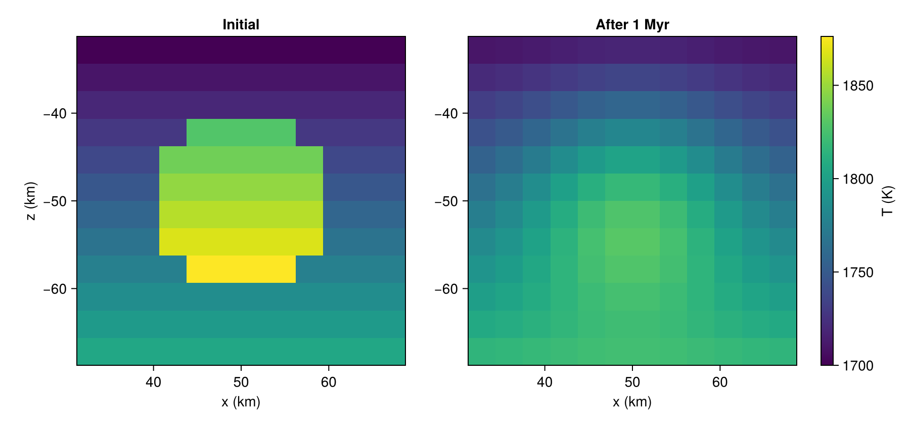
This page was generated using Literate.jl.