Fields

With a given grid that allows us to define each point uniquely in a high-dimensional space, we abstract the data values to be defined on the grid under the concept AbstractField. Following is the type tree of the abstract field and its derived data types.

Defining a multi-dimensional Field

Consider the following example, where we defined a variable grid of type Chmy.UniformGrid, similar as in the previous section Grids. We can now define physical properties on the grid.

When defining a scalar field Field on the grid, we need to specify the arrangement of the field values. These values can either be stored at the cell centers of each control volume Center() or on the cell vertices/faces Vertex().

# Define geometry, architecture..., a 2D grid
grid = UniformGrid(arch; origin=(-lx/2, -ly/2), extent=(lx, ly), dims=(nx, ny))

# Define pressure as a scalar field
Pr = Field(backend, grid, Center())

With the methods VectorField and TensorField, we can construct 2-dimensional and 3-dimensional fields, with predefined locations for each field dimension on a staggered grid.

# Define velocity as a vector field on the 2D grid
V = VectorField(backend, grid)

# Define stress as a tensor field on the 2D grid
τ = TensorField(backend, grid)

Use the function location to get the location of the field as a tuple. Vector and tensor fields are currently defined as NamedTuple's (likely to change in the future), so one could query the locations of individual components, e.g. location(V.x) or location(τ.xy)

Initialising Field

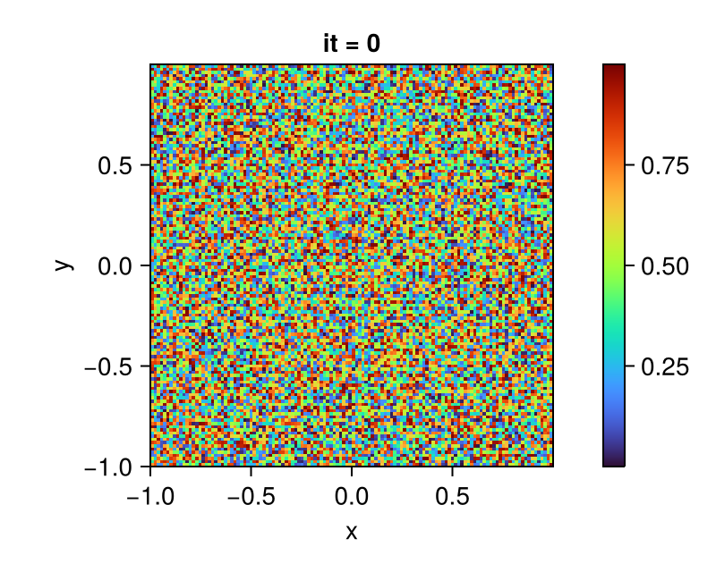
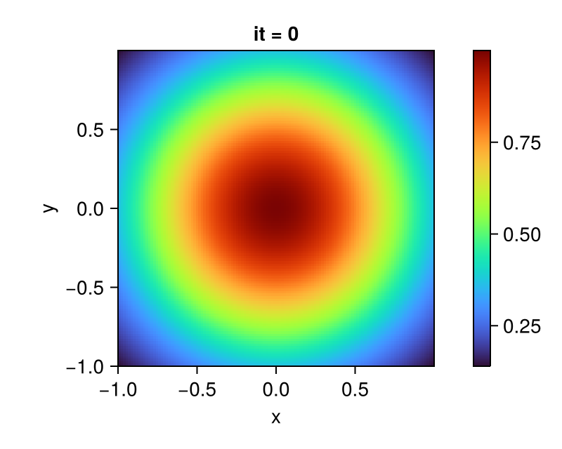
Chmy.jl provides functionality to set the values of the fields as a function of spatial coordinates:

C = Field(backend, grid, Center())

# Set initial values of the field randomly
set!(C, grid, (_, _) -> rand())

# Set initial values to 2D Gaussian
set!(C, grid, (x, y) -> exp(-x^2 - y^2))

A slightly more complex usage involves passing extra parameters to be used for initial conditions setup.

# Define a temperature field with values on cell centers
T = Field(backend, grid, Center())

# Function for setting up the initial conditions on T
init_incl(x, y, x0, y0, r, in, out) = ifelse((x - x0)^2 + (y - y0)^2 < r^2, in, out)

# Set up the initial conditions with parameters specified
set!(T, grid, init_incl; parameters=(x0=0.0, y0=0.0, r=0.1lx, in=T0, out=Ta))

Defining a parameterized FunctionField

A field could also be represented in a parameterized way, having a function that associates a single number to every point in the space.

An object of the concrete type FunctionField can be initialized with its constructor. The constructor takes in

1. A function func
2. A grid
3. A location tuple loc for specifying the distribution of variables

Optionally, one can also use the boolean variable discrete to indicate if the function field is typed Discrete or Continuous. Any additional parameters to be used in the function func can be passed to the optional parameter parameters.

Example: Creation of a parameterized function field

Followingly, we create a gravity variable that is two-dimensional and comprises of two parameterized FunctionField objects on a predefined uniform grid grid.

1. Define Functions that Parameterize the Field

In this step, we specify how the gravity field should be parameterized in x-direction and y-direction, with η as the additional parameter used in the parameterization.

# forcing terms
ρgx(x, y, η) = -0.5 * η * π^2 * sin(0.5π * x) * cos(0.5π * y)
ρgy(x, y, η) = 0.5 * η * π^2 * cos(0.5π * x) * sin(0.5π * y)

2. Define Locations for Variable Positioning

We specify the location on the fully-staggered grid as introduced in the Location on a Grid Cell section of the concept Grids.

vx_node = (Vertex(), Center())
vy_node = (Center(), Vertex())

3. Define the 2D Gravity Field

By specifying the locations on which the parameterized field should be calculated, as well as concretizing the value η = η0 by passing it as the optional parameter parameters to the constructor, we can define the 2D gravity field:

η0 = 1.0
gravity = (x=FunctionField(ρgx, grid, vx_node; parameters=η0),
           y=FunctionField(ρgy, grid, vy_node; parameters=η0))

Defining Constant Fields

For completeness, we also provide an abstract type ConstantField, which comprises of a generic ValueField type, and two special types ZeroField, OneField allowing dispatch for special casess. With such a construct, we can easily define value fields properties and other parameters using constant values in a straightforward and readable manner. Moreover, explicit information about the grid on which the field should be defined can be abbreviated. For example:

# Defines a field with constant values 1.0
field = Chmy.ValueField(1.0)

Alternatively, we could also use the OneField type, providing type information about the contents of the field.

# Defines a field with constant value 1.0
onefield = Chmy.OneField{Float64}()

Notably, these two fields shall equal to each other as expected.

julia> field == onefield
true