Getting Started with Chmy.jl

Chmy.jl is a backend-agnostic toolkit for finite difference computations on multi-dimensional computational staggered grids. In this introductory tutorial, we showcase the essence of Chmy.jl by solving a simple 2D diffusion problem. The full code of the tutorial material is available under diffusion_2d.jl.

Basic Diffusion

The diffusion equation is a second order parabolic PDE, here for a multivariable function $C(x,y,t)$ that represents the field being diffused (such as the temperature or the concentration of a chemical component in a solution) showing derivatives in both temporal $\partial t$ and spatial $\partial x$ dimensions, where $\chi$ is the diffusion coefficient. In 2D we have the following formulation for the diffusion process:

$$\frac{\partial C}{\partial t}=\chi (\frac{{\partial }^{2}C}{\partial x^2}+\frac{{\partial }^{2}C}{\partial y^2}).$$

Introducing the diffusion flux $q$, we can rewrite the above equation as a system of two PDEs, consisting of the following two equations,

$$\mathit{q}=-\chi \mathrm{\nabla }C,$$$$\frac{\partial C}{\partial t}=-\mathrm{\nabla }\cdot \mathit{q}.$$

Boundary Conditions

Generally, partial differential equations (PDEs) require initial or boundary conditions to ensure a unique and stable solution. For the field C, a Neumann boundary condition is given by:

$$\frac{\partial C}{\partial \mathit{n}}=g(x,y,t)$$

where $\frac{\partial C}{\partial \mathit{n}}$ is the derivative of C normal to the boundary, and $g(x,y,t)$ is a given function. In this tutorial example, we consider a homogeneous Neumann boundary condition, $g(x,y,t)=0$, which implies that there is no flux across the boundary.

Using Chmy.jl for Backend Portable Implementation

As the first step, we need to load the main module and any necessary submodules of Chmy.jl. Moreover, we use KernelAbstractions.jl for writing backend-agnostic kernels that are compatible with Chmy.jl.

CPUs

using Chmy
using KernelAbstractions # for backend-agnostic kernels
using Printf, CairoMakie # for I/O and plotting

backend = CPU()
arch = Arch(backend)

Nvidia GPUs

using Chmy
using KernelAbstractions # for backend-agnostic kernels
using Printf, CairoMakie # for I/O and plotting
using CUDA
backend = CUDABackend()
arch = Arch(backend)

AMD GPUs

using Chmy
using KernelAbstractions # for backend-agnostic kernels
using Printf, CairoMakie # for I/O and plotting
using AMDGPU
backend = ROCBackend()
arch = Arch(backend)

Apple GPUs

using Chmy
using KernelAbstractions # for backend-agnostic kernels
using Printf, CairoMakie # for I/O and plotting
using Metal
backend = MetalBackend()
arch = Arch(backend)

In this introductory tutorial, we will use the CPU backend for simplicity:

backend = CPU()
arch = Arch(backend)

If a different backend is desired, one needs to load the relevant package accordingly. For further information about executing on a single-device or multi-device architecture, see the documentation section for Architectures.

Metal backend

Metal backend restricts floating point arithmetic precision of computations to Float32 or lower. In Chmy, this can be achieved by initialising the grid object using Float32 (f0) elements in the origin and extent tuples.

Writing & Launch Compute Kernels

We want to solve the system of equations (2) & (3) numerically. We will use the explicit forward Euler method for temporal discretization and finite-differences for spatial discretization. Accordingly, the kernels for performing the arithmetic operations for each time step can be defined as follows:

@kernel inbounds = true function compute_q!(q, C, χ, g::StructuredGrid, O)
    I = @index(Global, Cartesian)
    I = I + O
    q.x[I] = -χ * ∂x(C, g, I)
    q.y[I] = -χ * ∂y(C, g, I)
end

@kernel inbounds = true function update_C!(C, q, Δt, g::StructuredGrid, O)
    I = @index(Global, Cartesian)
    I = I + O
    C[I] -= Δt * divg(q, g, I)
end

Non-Cartesian indices

Besides using Cartesian indices, more standard indexing works as well, using NTuple. For example, update_C! will become:

@kernel inbounds = true function update_C!(C, q, Δt, g::StructuredGrid, O)
    ix, iy = @index(Global, NTuple)
    (ix, iy) = (ix, iy) + O
    C[ix, iy] -= Δt * divg(q, g, ix, iy)
end

where the dimensions could be abstracted by splatting the returned index (I...):

@kernel inbounds = true function update_C!(C, q, Δt, g::StructuredGrid, O)
    I = @index(Global, NTuple)
    I = I + O
    C[I...] -= Δt * divg(q, g, I...)
end

Model Setup

The diffusion model that we solve should contain the following model setup

# geometry
grid   = UniformGrid(arch; origin=(-1, -1), extent=(2, 2), dims=(126, 126))
launch = Launcher(arch, grid)

# physics
χ = 1.0

# numerics
Δt = minimum(spacing(grid))^2 / χ / ndims(grid) / 2.1

In the 2D problem only three physical fields, the field C and the diffusion flux q in x- and y-dimension are evolving with time. We define these fields on different locations on the staggered grid (more see Grids).

# allocate fields
C = Field(backend, grid, Center())
q = VectorField(backend, grid)

We randomly initialized the entries of C field and finished the initial model setup. One can refer to the section Fields for setting up more complex initial conditions.

# initial conditions
set!(C, grid, (_, _) -> rand())
bc!(arch, grid, C => Neumann(); exchange=C)

You should get a result like in the following plot.

fig = Figure()
ax  = Axis(fig[1, 1];
           aspect = DataAspect(),
           xlabel = "x", ylabel = "y",
           title = "it = 0")
plt = heatmap!(ax, centers(grid)..., interior(C) |> Array;
               colormap = :turbo)
Colorbar(fig[1, 2], plt)
display(fig)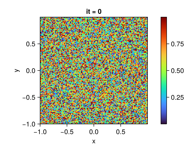

Solving Time-dependent Problem

We are resolving a time-dependent problem, so we explicitly advance our solution within a time loop, specifying the number of iterations (or time steps) we desire to perform. The action that takes place within the time loop is the variable update that is performed by the compute kernels compute_q! and update_C!, accompanied by the imposing the Neumann boundary condition on the C field.

# action
nt = 100
for it in 1:nt
    @printf("it = %d/%d \n", it, nt)
    launch(arch, grid, compute_q! => (q, C, χ, grid))
    launch(arch, grid, update_C! => (C, q, Δt, grid); bc=batch(grid, C => Neumann(); exchange=C))
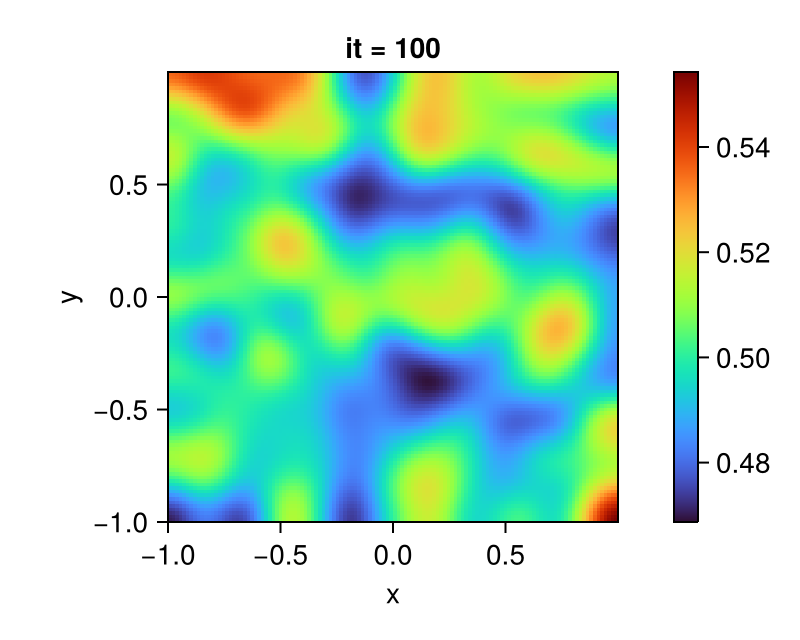
end

After running the simulation, you should see something like this, here the final result at it = 100 for the field C is plotted:

fig = Figure()
ax  = Axis(fig[1, 1];
           aspect = DataAspect(),
           xlabel = "x", ylabel = "y",
           title = "it = 100")
plt = heatmap!(ax, centers(grid)..., interior(C) |> Array;
               colormap = :turbo)
Colorbar(fig[1, 2], plt)
display(fig)